Frequency and Time Measurement

The measurement of time (and frequency) is something that we mostly take for granted, being used to watches and clocks from an early age. In fact it is a classic comparison of an unknown with a recognised ‘standard’. The early standard was the Sun, whose passage was noted and the interval between two ‘transits’ divided into 24 equal length ‘hours’. It was soon realised that the sun is a rather erratic standard and a complex way of averaging out the variations was devised, until finally in the 1960s the second was defined against an atomic transition of the caesium atom. It is fine to have a standard buried away in some academic establishment but it is necessary for many ordinary people to have access to the ‘standard’ for use in everyday life. This was achieved by the introduction of the watch and a technique for correcting it occasionally. The spread of the railways led to the need for a ‘universal’ time, constant over a country or at least a region. The clocks were able to be ‘synchronised’ by another invention widely used by the railways, the electric telegraph. This leads to the idea of making the ‘national’ standard available for use throughout the country.

History and Distribution of Time and Frequency Standards

The need for frequency to be measured accurately probably stems from the use of radio, though there was the requirement earlier to be able to tune musical instruments to a specified ‘pitch’. The initial standards for musical pitch were ‘pitch pipes’ and tuning forks. The pitch pipe depends for its note upon the resonance of a column of air inside a carefully made length of pipe. The tuning fork uses the mechanical resonance of a relatively heavy ‘fork’ of metal. In the early days of radio the tuning fork was re-engineered to be ‘electrically maintained’, by means of coils and an maintaining amplifier. A great deal of experimentation was necessary to allow for the effects of temperature which caused the fork to expand and it resonant frequency to drop. Eventually the forks were made of Invar, a very low expansion coefficient iron alloy, and where housed in a carefully controlled box., to minimise temperature variation and shock. The transmitting frequency of the Rugby LF station GBR , which transmit on 16kHz, was controlled in the early days (1920s) by this technique. Of course the elaborate arrangement was not a standard but simply a ‘local watch’ which needed to be ‘calibrated’ against the national standard occasionally. In the 1930s the quartz crystal resonator (and oscillator ) was perfected and a an immediate jump in the stability of local ‘timepiece was possible. In 1936 the then General Post Office developed a speaking clock with a sound system based on optical variable area recording as used in the cinema industry, but on glass discs. This was initially only available in the London area. The mechanism was driven by a 4Hz synchronous motor requiring so much power that transmitting valves were used in the amplifier supplying the power. This was synchronised to the time signal "pips" and was accurate to about +/- 100msecs. After W.W.II when magnetic recording became available the Post Office used a quartz crystal oscillator to maintain a speaking clock to very high accuracy for its time (+/- 1msec), and be readily available to anyone in the country with access to a telephone. The British Broadcasting Corporation’s transmitters started to be controlled by very stable quartz crystal oscillators, some later based on the ‘Essen Ring’ structure devised by Dr Essen who was responsible for the national time standard at the National Physical Laboratory (NPL). The Essen Ring produced a resonator with a very high ‘Q’, but is was a very fragile construction and needed to be treated with great care. The Post Office Radio station at Rugby started to transmit standard frequencies in the 1950s, and in the 1960s these transmissions where stabilised to a high degree using Caesium oscillators. At about the same time the longwave broadcast Station of the BBC at Droitwich, then transmitting on 200kHz ,was also stabilised by a caesium oscillator. These stations provided a traceable standard to the whole of the UK. Absolute measurements of Rugby and Droitwich are posted every month by NPL.

We now have easy availability to a standard, how best do we use it to calibrate our local equipment?

The simplest technique has been used by piano and other musical instrument tuners for years. It involves the use of ‘beats’. These are the difference frequencies that can be heard when two audible tones are tuned close to each another. At first a low audio note can be heard, then as the difference drops below the lowest audible frequency this ‘beat’ will cause the sound of the tones to slowly swell and fade. If the time between the swell peaks is ten seconds the frequencies are within 0.1Hz of each other. With musical instruments it is also possible to hear these beats on harmonics as well, making it possible to tune and instrument completely with just one standard fork, or pitch pipe.

Similar techniques can be used for electronic oscillators, by utilising an audio amplifier and speaker of a radio receiver. In the days when MSF transmit a standard on 10MHz it was possible to tune it in on a receiver, and then by coupling some of a local 10MHz oscillator into the receiver adjust the calibration capacitor on the local oscillator until the beat was inaudible. A further improvement could be achieved by switching on the BFO in the receiver to produce a moderately high audio tone. The beat between the MSF signal and the local oscillator then caused the beat tone to swell and fade. This "three-signal technique" was very popular before the days of frequency counters. It was easy to adjust the local oscillator to within 0.1Hz of the MSF standard. It was not worth going further than this as the ionospheric effects in the propagation of the MSF signal degraded the accuracy to about 1 part in 10^8. A part in 100 million is quite good enough for a lot of applications including most of amateur radio. If the 10MHz local signal was the ‘timebase’ oscillator in your frequency counter, you now had that level of accuracy in all measurements made with that instrument. How long after the calibration you could rely on it ,we will consider later.

The Heterodyne Frequency Meter

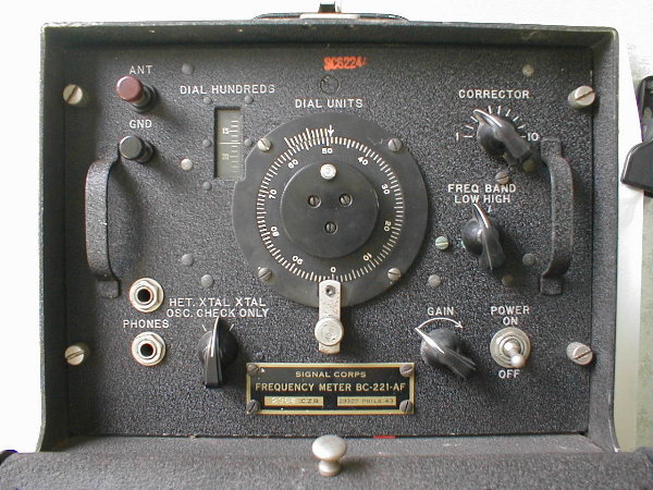
How on earth did we measure odd frequencies accurately before counters were available in the late 1960s. (professional units available in the early 1960s from firms like Schomandel, Racal, Solartron and Cintel, were very expensive monsters.) Well, by using beats, of course ,and an interpolation oscillator. The package containing a local ‘standard ‘ , a quartz crystal oscillator, and an interpolation oscillator was known as a heterodyne frequency meter. By far the most famous of these, certainly to radio amateurs, but to many professionals as well, was the ex-US-military unit carrying the designation BC-221 (or SCR-211). Similar units were produced for the UK military, but the BC-221 became the ‘gold standard’ for amateur frequency measurement.

The BC-221 has an internal variable frequency oscillator (VFO) with a lockable vernier dial, and under the transparent window on the front flap is a calibration table. The first thing to check is that the typewritten serial number on the front page of the calibration chart agrees with the serial number on the plate on the lower front of the front panel. If it does the table is usable, if not the table is for scrap as it refers to the inner construction of another unit, and the calibration tables were individually produced for each unit. It is not an absolute disaster as a new calibration table can easily be re-constructed (*).

The BC-221 contains a 1MHz crystal oscillator and an LC VFO with two switched ranges. The two oscillators are fed to a mixer and the beat note is made audible in headphones. The calibration depends on the fact that there are a multitude of VFO frequencies that will produce an audible beat with the crystal oscillator. These are the mth harmonic of the crystal with the nth harmonic of the VFO. The value of m+n is referred to as the ‘order’ of the beat and the lower the ‘order’ the louder the beat note will be. It is possible to detect beats for every few kilohertz shift of the variable oscillator. If we know the approximate frequency of the VFO, we can accurately calculate the frequency of the VFO at nearest ‘zero beat’ . These are recorded as cardinal points in the table. If the points are close enough together, then it is sufficiently accurate, for most purposes, to linearly interpolate the dial readings between two adjacent ‘beat’ points. Thus a complete table of frequency settings can be compiled. I believe that in the 1940s the process was speeded up by having several hundred operators, who set the dials for fixed frequencies that piped round the room to all of them , and they recorded the dial setting vernier for their instrument. Then individual tables were calculated from these values and individual calibration books were printed for each instrument. According to some reports a more fully automated procedure was installed in mid-1942 at most of the factories, but I have seen no contemporary description of this. With the advent of personal computers it may be possible to improve a little even on that technique.

Now we have a unit with a calibration table there are several steps that need to be taken to use it for frequency measurement. First the crystal which is the internal standard, was made many years ago and, though adjusted at the factory, may not still be resonating at exactly 1MHz. We need to trim the internal crystal oscillator into calibration with an off air standard. This was best done when the HF transmissions were still being made, by tuning a receiver to 10MHz MSF (or WWV) and adjusting the crystal to zero beat using the three oscillator method outlined above. It was possible to get a beat drift of longer than ten seconds which indicates that the 1MHz local ‘standard’ is within 1 part in 100 million of the national standard. There is no point in trying to improve on this as the temperature stability of the crystal and valve oscillator are not good enough to maintain the higher accuracy for very long. Also the accuracy of the short-wave distribution signals is limited by the effects of ionospheric ‘reflections’. The crystal trimmer is hidden to prevent ‘unauthorised’ twiddling by curious ‘squaddies’. You can access it by removing the four screws holding the serial-number plate. The next stage is to select the range of the VFO ( HIGH or LOW ) that covers the frequency we wish to measure, and open the calibration table at the appropriate page. At the bottom of each page there is given a "crystal check point" with a dial setting. This is the beat point that validates this page. Set the dial to the reading quoted and select "CRYSTAL CHECK" on the function switch, then adjust the "CORRECTOR" on the top right for a zero beat in the headphones. You can now measure an external source by switching the function switch to "HET OSC", coupling the signal into the BC-221 via the telescopic aerial or the terminals and adjusting the dial for zero beat, reading off the vernier, and translating that to a frequency with the table. Alternatively you can set the vernier dial to a required frequency and inject the signal to a receiver, so that the receiver will be exactly on the channel of an expected transmission.

There are problems with this procedure and it does need to be used with some skill. The use of the BC-221 assumes you have a receiver and know approximately what the frequency is. It is possible of course to get a multitude of beats when measuring an external source, but you are expecting a low order beat and it will be very loud. Once again you should know the approximate frequency. The BC-221 and its lesser known brethren allowed RT operators with only a rudimentary knowledge of electronics to set up and operate nets, and to meet schedules with minimal calling. It was so good that the Russians, who presumably received units via Lease-Lend, were so impressed they manufactured a copy.

The stability of the BC-221 VFO was such that it was used as a standby excitation unit in the HF station at Rugby. If a crystal source failed or a transmission had to made on an unusual frequency the ‘221 was there to be pressed into service. I saw one in this position on a visit to the station in about 1962. Synthesisers were becoming available at the time but filled a room !! There were also several articles written in the ARRL’s QST after in the late 1940s describing the use of the BC-221 as a Variable Frequency Oscillator for transmitter control.

Frequency Counters

Of course nobody would use such a archaic method of measurement now......or would they? Everyone uses digital reading equipment now, but some of the same principles still apply. Your digital frequency counter is only as good as the local timebase standard. Many cheaper counters have a simple 10MHz crystal oscillator, which is used to generate the counting or gate periods. Cheap quartz crystals have a temperature coefficient of about 1 part per million per degree Celsius. So if set up at 20 degrees you could be anything up to 5Hz per MHz in error just due to temperature changes. Quartz crystals change (upward) in frequency from the time they are manufactured, this is known a ‘ageing’. The greatest ageing change occurs early in the use of the crystal. After about 12 months in use the ageing rate settles down to an almost constant value. The actual rate depends very much on the quality of the crystal and its enclosure. A good temperature controlled crystal oscillator will have an ageing specification of about 1 part in 1000 million per year (e.g. a Racal 9420, as found optionally installed in many of their better counters). If one of these is fitted to your counter and adjusted with reference to Rugby or Droitwich, you should be able to measure accurately to about 1 Hz at 70cms frequencies. Then some care is needed with the measurement. If the signal you are measuring has a high harmonic content it may be possible to get an erroneous reading, because of the highly distorted waveform.

The accuracy of a counter is usually stated as the accuracy of the timebase source +/- 1 count. Because the opening of the timer gate is random compared with the phase of the unknown signal, we may count differently on successive periods. This has been referred to as "last digit jitter" as is upsetting for some, who would like to see a clearly defined answer. However it can be used to increase the resolution (note, NOT the accuracy ) of the counter. For example if we have a 6-digit counter, and we read a count of 700405 with the last digit wavering between 5 and 6. If we count the number of times the count ends in 5 out of ten samples we can effectively add an extra digit to the frequency readout. Thus if we have three 5s and seven 6s, the frequency would be 7004057. This is a statistical increase in resolution and depends on the relationship between the start of the gate period and the signal phase being totally random. The more samples averaged the more accurate it should become. Another way that you can sometimes increase the resolution is by over-ranging. this means selecting a gate period that will cause the display to over-fill or overflow. If the gate period is lengthened until the first digit ‘falls off the left hand end of the display’ the remaining digits are usually still correct and we have an extra digit of resolution. The significance of this higher resolution is determined by the accuracy of the timebase. Just because you have 8 digits displayed does not necessarily mean that the extreme right-hand one has any real meaning. Many modern counters will not over-range in this way.

The above discussion leads us one to two aspects of accuracy of a frequency source, the long term stability and the short term stability. The short-term stability of a standard frequency distributed by radio may not be good because its reception may be affected by noise or propagation variation. If we make sure to compare our local standards with it over a relatively long period of time these random fluctuations will average out and we will see almost the accuracy of the controlling source. If we are making measurements with a gate time of one second, we do not want a timebase source that is moving around on a second-by-second basis. (this can be thought of as random frequency modulation of the timebase oscillator). Thus the specification for a high grade frequency counter calls for an oscillator with a good short-term stability. This is usually achieved with a carefully cut, high-grade crystal which is enclosed in a temperature controlled environment or ‘oven’ (OCXO). A slightly cheaper option is a temperature-compensated crystal oscillator (TCXO). The long term performance is not quite so important as it can be re-aligned with a standard periodically to achieve the required overall accuracy.

Multiplying the Error

If one has a standard and an unknown that are very close together it can take a long time (the beat note may have a period of days !!) to acquire a comparison between the two and so a calibration of the unknown. I saw the following system used in the early 1960s for investigating the short term stability of oscillators, and quickly aligning oscillators to a standard.

Assume the standard is at 1MHz and the unknown is at (1+df) MHz where df is the (small) error. The unknown is multiplied by 10, and then mixed with 9 times the standard. The filtered output from the mixer is (1+ 10*df)MHz. This was done 3 times , but the final time it was mixed with 10 times the standard. The output from the system was 1000 times the frequency error. In the instrument I saw, it was used to drive a recorder which was continuously indicating very small phase changes against time. It occupied a 3metre run of lab bench !! Since that time I have recently come across units called Frequency Difference meters made by Tracor and Montronics ( later Fluke, Keithley, and Adret I believe) which use just this system of error multiplication. The limitation is that the incidental phase noise is also multiplied up, and the limitation is probably around the 1000 to 10,000 times. The final display can be a phasemeter, or the Montronics gives quadrature outputs that can produce Lissajous figures of the multiplied "beat". If we use this, it may be possible to use the scope writing speed limitation to act as a averager and overcome some of the multiplied noise problems.

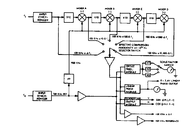
Block diagram of the Fluke Model 103

Quartz Crystal Limitations

As far as I can ascertain there are several causes of ageing. I had described to me an experiment where a natural quartz blank ( all crystals before about 1965 were cut from natural quartz crystals. since that time synthetic quartz, or more correctly artificially grown crystals, have been used ) was placed between two plates with several kV across the crystal. The whole assembly was heated up to several hundred degrees Celsius for a few days, and at the end of that period the plates were covered in contamination that had been driven out of the quartz. Contamination trapped in the crystal lattice is also able to migrate when the plate is vibrating.

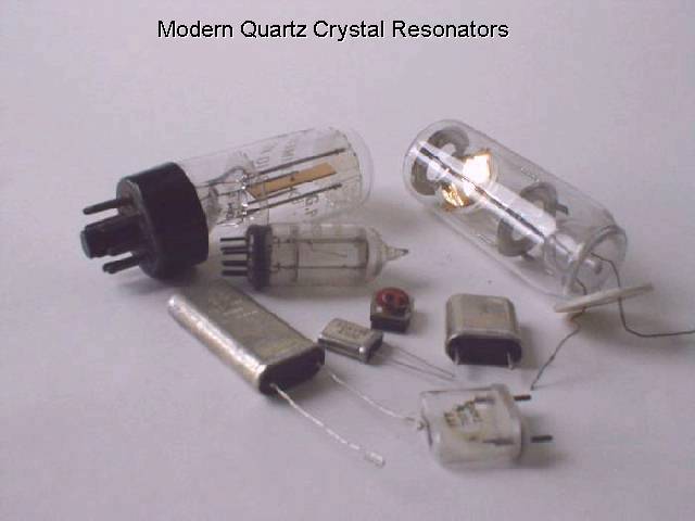
The ‘synthetic’ crystals, like the one pictured above, are grown from a ‘seed’ crystal dipped into a crucible of melted very pure silica, and so there is less internally trapped contaminant. You can just see the wires which held the 'seed' plate. The facets are the facets seen on natural quartz crystals. Also when quartz crystals are finished the grinding process leaves a thin layer of slightly damaged, or imperfect lattice. Over time with the mechanical forces of the oscillation small quantities of this are shed from the crystal surface, hence the ageing is usually upward in frequency. This last effect is circumvented in high quality crystals by polishing to a very fine finish. The ‘damage’ layer is a function of the grit size used for the last lapping or polishing stage. High quality crystals used to be finished with 1/4 micron* diamond paste. Then to remove the last levels of damage the crystals were lightly etched in hydrofluoric acid.

* 1 micron is 1/1000000th of a metre or 1/1000th of a mm.

Next the electrodes which are usually applied by vacuum sputtering or vacuum evaporation or either aluminium or gold. Aluminium is reactive and keys well to the quartz, but will oxidise if any remaining air is present. It is also cheap and easy to evaporate, or sputter, as it has a melting point around 640 degrees Celsius. Gold is expensive and whilst it adheres well to quartz , but requires a temperature over well over the melting point of 1060 degrees Celsius. In both cases it is possible to trap molecules of gas in the electrode layer. Sputtering is more lightly to do this as it takes place in an inert gas at a higher pressure than the evaporation process.

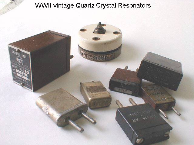
The final quality of a crystal can often be judged by the type of holder it is mounted in. Solder sealed crystal cans may suffer from impurities from the flux and the soldering process condensing on the crystal. Resistance welded cans are better as there is no flux, but the seal does reach a high temperature and gasses may released. Cold-welding where the flanges are pressed together until the metal in the two sections of the enclosure flow together is the best enclosure for a stable high quality unit. Glass encapsulation is somewhere in between these. The crystal may be mounted in a vacuum or an inert gas, but the final sealing requires a flame to melt the glass components together so there can be some contaminant release. Most of the high quality crystals I saw that were made in the late 1950s were mounted in glass enclosures familiar to vintage radio enthusiasts as the International Octal GT format.

I believe that most of the crystals used for high quality ovened standards at that time were plano-convex or ‘lens-shaped’, and operated on their third overtone at 5MHz. I have seen ‘Q’ values quoted for units at that time of over one million, and believe approaching 5 million for the best units. Great care was taken to use the minimum drive power to avoid any heating of the crystal, and the drive level was stabilised in a bridge circuit which use a filament lamp as one of the ratio arms. This circuit, the Meechan Bridge oscillator, is not much seen these days. The highest quality standards were mounted in triple temperature controlled oven where the crystals was maintained accurately to within one milli-degree Celsius. Really high quality crystals are now SC cut, and units are even being made with no metal electrodes or suspension. The crystal is supported on a quartz ring with support "pips" and the coupling to the crystal is all capacitive. These are highly expensive units and would probably cost several thousand pounds (sterling) each, I suspect they are also rather fragile. Their advantage is that they do provide very good short term stability. Quartz will be with us for some time to come.

Comparing Frequency Standards with an Oscilloscope

As you may have noticed from the above discussions most standards are in the 1 to 10MHz range. If we use a three signal beat technique to compare these, then the best we can really hope for is about 1 in 10,000,000 to maybe 1 in 100,000,000 for 10Mhz and a 10 second swelling beat. It is possible to do a little better than that by using an oscilloscope and it may also be possible to compare standards that are at different frequencies.

The technique probably works best if one of the signals are squared up. This could be the off-air standard locked to Droitwich for example. The squared signal is used to trigger the oscilloscope with the trigger setting on external. The local standard (say a 1MHz output from your counter) is applied to the Y1 input. The timebase is adjusted to 0.1usec/division. You should see a single cycle of the local standard slipping slowly across the scope tube-face. The rate of this slippage is the ‘beat’ between the two signals. You can now adjust the counter clock to bring the trace as near stationary as possible. You then note the position of the end of the cycle, this is exactly 1 usec. Time (with a simple stopwatch) a point on the waveform until it has slipped one whole cycle. If that takes 100 seconds then the counter timebase is within 1 part in 100,000,000 of the national standard. What is more, with a little thought you can determine whether the counter crystal is oscillating higher or lower in frequency than the standard. Do not worry if you can not get the trace perfectly stationary, surprisingly enough it is better if there is a slight difference, it makes the measurement easier. Because the local standard will not remain perfectly in synchronism with the national standard it is sufficient to know what its error is at a given point. If the two standards are very close it will take a very long time to produce a cycle of the beat If the slip is very slow it is possible to time the slip over a tenth of a cycle (100nsecs) and make the measurement more quickly. This method has the advantage that the measurement is made over a relatively long ‘averaging’ period so the effects of any modulation on the ‘standard’ carrier will not be seen. Fluke now make a meter working on a similar principle or measuring the time interval between two signals at two widely spaced points in time. You will find this described in one of the 2003 Time and Frequency Club newsletters. If more accuracy is required it may be necessary to log the phase drift using a phase meter and datalogger over a period of an hour of more and make small corrections (a manual PLL !!) Your requirement will depend upon the stability of your local standard. There is no point it trying to set it to a higher order than it is capable of holding over a few weeks. Often it is better to attach a label to an instrument detailing the "offset" rather than trying to set it accurately. Most good ex-commercial counters and synthasisers can be set to about 1 in 10^9, but many lower grade instruments will not hold that level of accuracy for long. Many cheap counters can be made very accurate by inserting an high grade external standard signal.

There are other techniques that can be used and everyone seems to know about Lissajous figures. These can be very useful but are a bit cumbersome and one definitely needs to time a complete rotation to be sure. It is probably best to time from a 0 degree phase point (a diagonal line) to the next 180 degree phase point (a diagonal line sloping the other way). This is a half cycle slip. Selecting the exact timing point is not as easy as timing the trace slip past a fixed point on the scope tube-face Another somewhat easier technique is described in Scroggie’s Radio laboratory Handbook, which consists of making a simple circular timebase, and having the unknown produce a cog-wheel effect. This method was most useful when it was necessary to synchronise harmonics, to build a frequency calibration chart.

A further simple technique ( devised by G4GVW) that can be used with a dual beam oscilloscope is to put the two sources on to the Y1 and Y2 inputs, trigger can be ‘AUTO’ and either input. Then view the trace with the ‘ADD’ ( and optionally the ‘INVERT’ ) function activated. The trace now contains a "squiggle" that is a function of the phase difference between the two signals. The squiggle will seem to run along the trace, and you can zero in by adjusting the local signal so that the squiggle becomes stationary. This one works best with near sinewave signals.

Available Standards

The most obvious standards were the radio transmissions, in the UK the callsign is MSF. Unfortunately the high frequency transmissions at 2.5, 5 and, 10 MHz ceased some time ago, so now the most readily available is the Droitwich transmission on 198kHz ( BBC Radio 4 ). There are a number of commercial ‘Off-Air’ locked frequency standards that use this transmission to produce 1, 5 and 10Mhz outputs, with an accuracy close to the caesium-locked controlling oscillator. There are also several articles in the hobby magazines describing the construction of such a unit. At least two units are available in the UK from Halcyon and Quartzlock. Both of these offer as an alternative the French station Allois on 162kHz which is also controlled by a cesium locked source. I believe these transmissions do not run the full 24 hours every day.

Another possible source which is available is the 60kHz MSF transmission from Rugby ( This is due to move to Anthorn on the Firth of Forth in April 2007. see the NPL site for more detail ). This carries time code modulation, but over a reasonable sample period this produces no error in the frequency. The 16kHz Rugby transmitter GBR used to carry time signals and was stabilised for use in the Omega navigation chain. Sadly this service closed in April 2003 (see my History of Rugby elswhere on the site) The Northern Europe Loran System chain of high power transmitters on 100kHz are all Cesium locked, but the future of this source is in doubt as it has be eclipsed by the satellite Global Positioning System (GPS). It is possible it may continue in service, also transmitting a differential correction signal for GPS. Finally and probably potentially the most accurate is the GPS system itself. We need to define "accuracy" a little more carefully here. The short term accuracy of GPS may not be as good as a good counter timebase over period of 1second. This is called short term accuracy. However averaged over a long period the accuracy of GPS appraoches that of the cesium standard. Each satellite carries a cesium clock and there is complex calculation done within the receiver to allow for the satellite parameters, and their effect on the transmission, and other known perturbing factors. The GPS receiver outputs a 1 second ‘tick’ which is "accurate" to about 20nsecs (since the removal of S.A.) on average. Thus it is necesssary to have a good crystal or rubidium standard for the short term stability and to "disciplin" this to follow the long term stability of the GPS standard. A skeleton GPS receiver PCB can be obtained for under £100 (as little as £10 on eBay in Dec 2006 ) which will form the basis of a very accurate time and frequency standard. Most of the world's digital telephone transmission systems seem to use the GPS timing for the master synchronisation. A number of articles have been written in the hobby magazines describing standards based on the GPS receiver.( 15 ) ( 16 ) ( 17 )( 19 )

It has been suggested that some TV Broadcast authorities distribute a ‘ MASTER SYNC ’ signal which is controlled by a cesium standard. Certainly there have been a number of articles which have used the horizontal sync signal from a working TV (which is tuned to a signal, and so locked) and locking a 1MHz crystal oscillator to it. This is quite convenient as the horizontal scan frequency for 625 line systems is 15.625kHz which just happens to be 1/64 MHz. At first sight this looks a good and easy option, because most people are within range of a TV transmitter that will lock up the set. The problem is knowing which networks do distribute a good traceable sync signal (The BBC does or did). There is now another effect which makes this source less useful. The ‘Master Sync’ distribution was necessary when programs were sent to the transmitters over an analogue link. It means that there is not a momentary picture roll, when switching from one program source to another. In more recent years the distribution of program material around the country has moved very much to digital links where the frame and line synchronisation is not so important. This unfortunately means that the pedigree of the line sync signals, as referenced to the national standard, may be doubtful at the highest level.

The above is not intended at address the the ultra high accuacy measurements of frequency and time that are possible. For that purpose I can do little better than refer you to the web site of Tom Van Baak (who's exploits were recently mentioned in Scientific American) http://www.leapsecond.com/ and the fund of expertise that is daily disseminated on the Yahoo Time-nuts Group. If you are interested in resolution of better than 1 part in 10^10 this is the place to go for information.

References

1. "Frequency Standards and Clocks: A Tutorial Introduction" , NBS Technical Note 616 (revision 2d) pdf copy referenced in the Contents
2. Klein "Atomic Frequency Standards and Standard Frequency Transmitters", VHF Communications 2/1978
3. War Dept. Technical manuals, " Frequency Meter Sets SCR-211-A,.....,AL" TM 11-300 ( for BC-221)
4. "Frequency Meters as Master Oscillators", QST, August, 1946, pp. 34 ff.
5. "The BC-221 Frequency Meter as a VFO", QST, March, 1947, schematic on p. 44
6. " A VFO amplifier for the LM Frequency Meter " (or similar), QST, January, 1950, pp. 20 ff.
7. * Using the BC-221 Frequency Meter at V.H.F.", QST, January, 1950, pp. 46 and 120
8. "Get MORE from your LM and BC-221 frequency meters", Radio-Electronics, August, 1962, pages 63, 64, and 66.
9. "Solid-State BC-221 Frequency Meter", QST, February, 1977, pages 35 & 36.
10, "Feedback" for the above on page 39 of QST, April, 1977.
11. "More on Solid-State Conversion of BC-221/LM Frequency Meters" on page 59 of QST, December, 1979.
12. "Notes on the BC-221" H.W.Gordon, CQ Magazine Aug. 1962, pp 52-56
13. "Calibrating the LM Frequency Meter" G.L.Countryman, QST Sept.1965, pp18-20.
14. "Frequency Measurement with the LM/BC-221" K.N.Sapp, QST, Sept. 1965, pp28-31
15, "High stability Frequency Standard" Wrigley. D., available on web site at address
http://www.microwave.fsnet.co.uk/projects/projects-2.htm
16. Schneider & Richter, "High Precision Frequency Standard for 10MHz" VHF Communications, 4/2000 and 1/2001
17, "A GPS based Frequency Standard", Brooks Shera, QST July 1998, pp 37-44
see also updates at http://www.rt66.com/index_fs.htm
18. "MSF Locked Frequency Reference" Andy Talbot (G4JNT), Radio Communication (RSGB), Apr/May 1994
19 "Simple GPS disciplined oscillator" http://www.g4jnt.com/SimpleGPSDO.htm using the Rockwell Jupiter GPS by Andy Talbot G4JNT
19. Scientific American. September 2002 Special Issue on " TIME" with a very good summary of the mileposts in clock development
20, "The Quest for Accuracy", Jens Nickel , Elecktor Electronics, January 2007 pp 28-32